Excel表格中如何制作圆锥图表？制作圆锥图表的方法

勤哲Excel服务器

软件大小： 73 MB

更新时间： 2016-11-24 21:34:21

所属分类： 办公工具

查看详情

yesky

标签：

• 勤哲
• Excel

  Excel表格中如何制作圆锥图表呢?下面就跟随小编一起来学习制作圆锥图表的方法，熟悉一下它的操作流程吧。

  一、制作条形统计图：

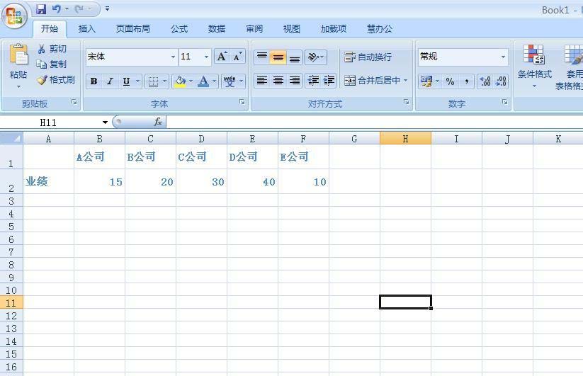
  1、打开Excel软件，如图所示，制作一组数据。

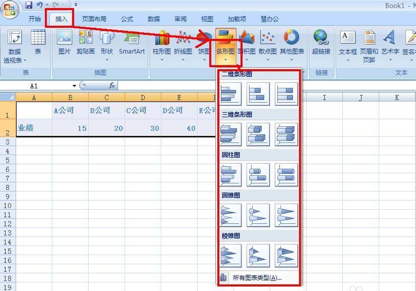
  2、选择数据区域表格，单击菜单栏“插入”——条形图，在“二维条形图”“三维条形图”“圆柱图”“圆锥图”“棱锥图”中选择一种条形统计图。

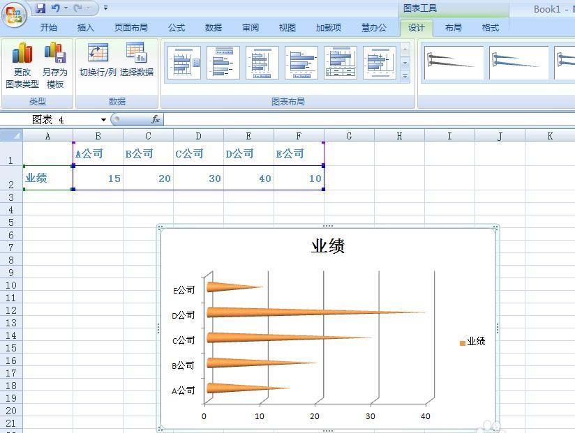
  3、现在就可以看到条形统计图制作好了，如图所示(这里选择了圆锥图)。

  二、编辑条形统计图：

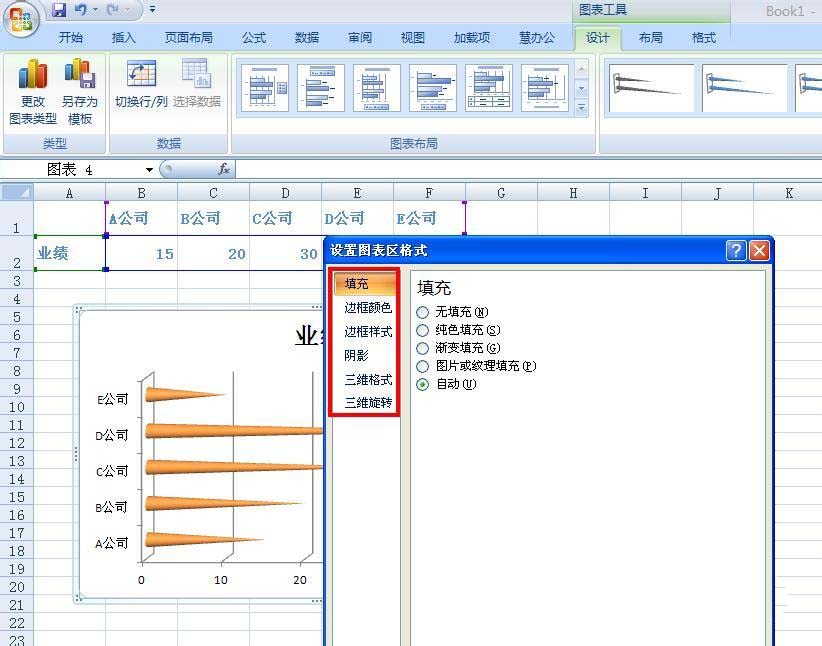
  1、设置图表区域格式

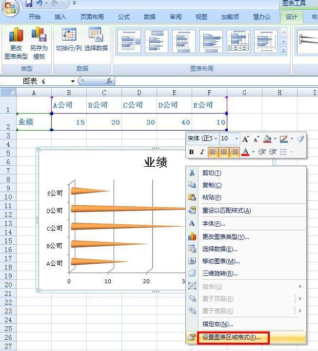
  在条形统计图的空白区域单击右键选择“设置图表区域格式”。

  在弹出的“设置图表区域格式”对话框中可以进行“填充”“边框颜色”“边框样式”“阴影”“三维格式”“三维旋转”的设置。

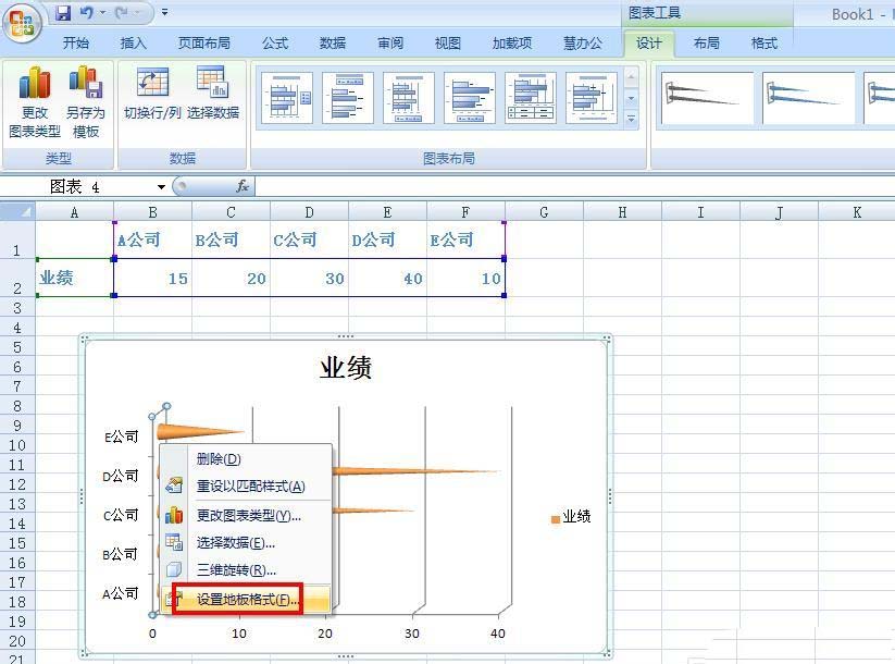
  2、设置地板格式

  在条形统计图的左边地板区域单击右键选择“设置地板格式”即可完成对地板的设置。

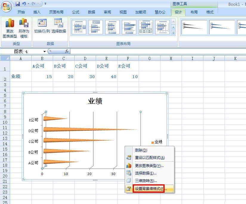
  3、设置背景墙格式

  在条形统计图的背景墙区域单击右键选择“设置背景墙格式”即可完成对背景墙的设置。

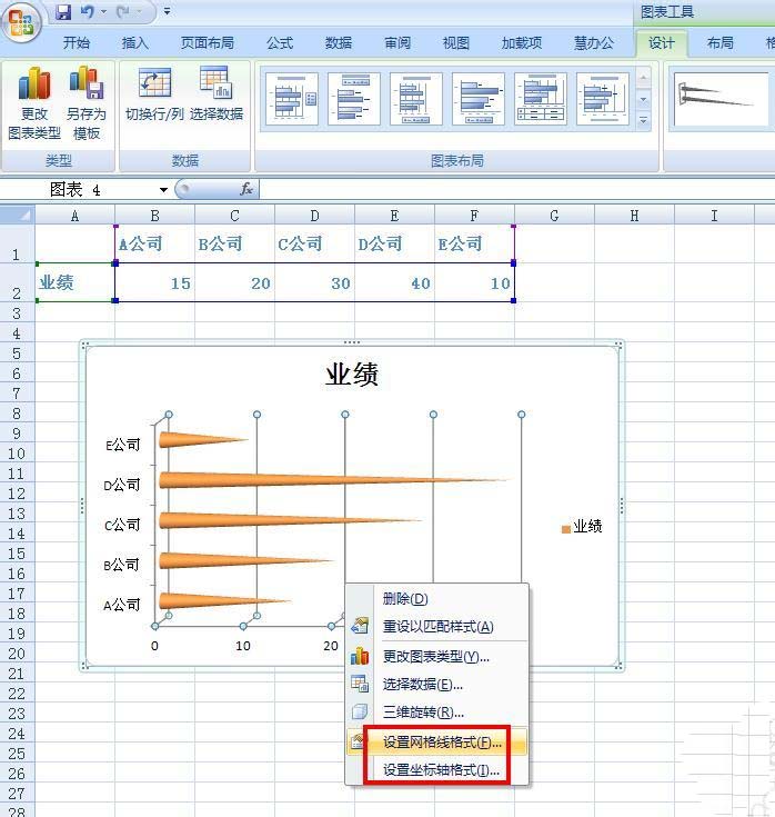
  4、设置网格线格式/设置坐标轴格式

  在条形统计图的网格线上单击右键选择“设置网格线格式/设置坐标轴格式”即可完成对网格线/坐标轴的设置。

  5、设置数据系列格式

  在条形统计图的数据点上单击右键选择“设置数据系列格式”即可完成对设置数据系列格式的设置。

  以上就是Excel表格制作圆锥图表的方法，希望可以帮助到大家。