excel2013如何制作柏拉图？excel2013制作柏拉图的方法

  excel2013如何制作柏拉图?柏拉图是我们工作中常常需要用到的，不会制作的赶快来看看excel2013制作柏拉图的方法吧。

  excel2013柏拉图制作教程：

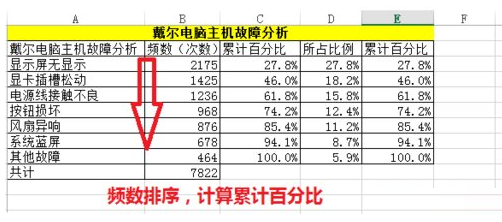
  制作柏拉图步骤1：如图所示，频数排序，计算累计百分比。图表制作使用前3列数据。

  制作柏拉图步骤2：选中数据区域——点击插入——推荐的图表——簇状柱形图。

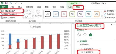
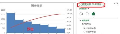
  制作柏拉图步骤3：点击图表工具(格式)——系列“累计百分比”——设置所选内容格式——次坐标轴。

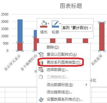
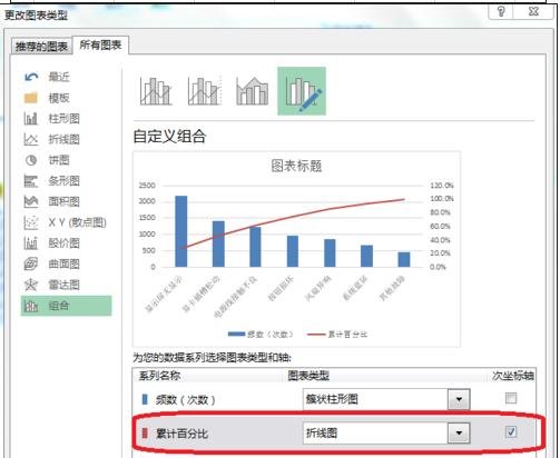
  制作柏拉图步骤4：右击——更改系列数据图表类型——累计百分比(折线图)。

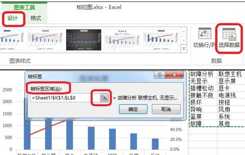
  制作柏拉图步骤5：点击图表工具(设计)——选择数据——轴标签区域(如图所示，把原来的拆分成两列，是柏拉图的横坐标轴的数据显示如图所示)

  制作柏拉图步骤6：调整分类间距

  制作柏拉图步骤7：如图所示，双击——设置数据系列格式——分类间距(0)。

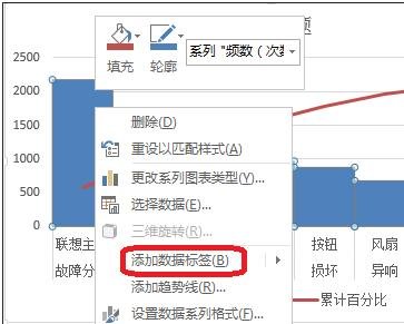
  制作柏拉图步骤8：右击——添加数据标签

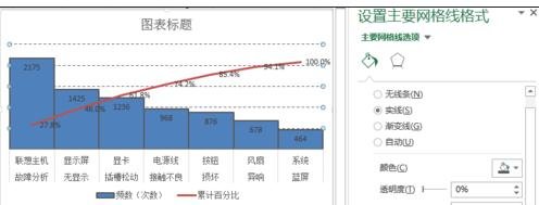
  制作柏拉图步骤9：双击网格线进行设置，如图所示。

  以上就是excel2013制作柏拉图的方法，希望可以帮助到大家。